Difference between revisions of "S16: Number 1"
Proj user17 (talk | contribs) (→Schedule) |
Proj user17 (talk | contribs) (→Grading Criteria) |
||
| (71 intermediate revisions by the same user not shown) | |||
| Line 1: | Line 1: | ||
| − | === | + | == Number 1 - Open CV Lane Departure == |
| − | |||
| − | |||
| − | |||
| − | |||
| − | |||
| − | |||
| − | |||
| − | |||
| − | |||
| − | |||
| − | == | + | == Abstract == |
| + | Drivers are in danger every day on the road. Changing lanes without notifying other drivers on the road will result in car accidents. Unsafe lane change is one of the top causes of car accidents on the freeway. In order to avoid car accidents by merging safely, drivers can: | ||
| + | |||
| + | 1) Always use the blinkers or turn signals. | ||
| + | |||
| + | 2) Only change one lane at a time. | ||
| − | + | 3) Never change lanes in an area where the lanes are separated by solid lines, only do so around dotted lines. | |
| − | This | + | |
| + | |||
| + | This system is built on top of OpenCV with computing capability on detecting the lane and provide a warning signal to the driver when they are about to be in danger. With the use of computer vision, the system will detect the current driver lane and provide a visual warning to the driver if no blinkers or turn signals is activated. | ||
== Objectives & Introduction == | == Objectives & Introduction == | ||
| − | + | The goal of this project is to deliver a lane warning system using OpenCV. If the driver is about to make a lane change, the system will calculate the departed percentage and warn the driver if they are in danger. | |
| + | |||
| + | '''OpenCV library and algorithm Overview''' | ||
| + | |||
| + | '''Color Spaces:''' This is a function to convert the original color to gray and HSV. | ||
| + | |||
| + | '''IPM (Inverse Perspective Mapping):''' IPM transforms the perspective of 3-D space into 2-D space. | ||
| + | |||
| + | '''Contours:''' Contours is to detect lane markings based on color and shape detection. | ||
| + | |||
| + | '''Gaussian Blur:''' Gaussian Blur is a diverse linear filter to smooth image on OpenCV. This is to smooth out edges and gets rid of unwanted noise. | ||
| + | |||
| + | '''Sobel Edge Detection:''' Sobel Edge ia an OpenCV to calculate the derivatives from the source. | ||
| + | |||
| + | '''Canny Edge Detection:''' Canny Edge detector is an OpenCV function to 1) Lower error rate 2) Better localization, and 3) Minimal response. | ||
| + | |||
| + | '''Hough Transform:''' The Hough Line Transform is a transform used to detect straight lines. This can be used after first edge detection processing. | ||
| + | |||
| + | '''Percentage offset:''' The percentage offset is used to determine how far away the center of the vehicle is from the center of the lane. | ||
| + | |||
| + | |||
=== Team Members & Responsibilities === | === Team Members & Responsibilities === | ||
| Line 39: | Line 56: | ||
! scope="col"| Status | ! scope="col"| Status | ||
! scope="col"| Completion Date | ! scope="col"| Completion Date | ||
| − | |||
|- | |- | ||
! scope="row"| 1 | ! scope="row"| 1 | ||
| Line 46: | Line 62: | ||
| Completed | | Completed | ||
| 3/20/2016 | | 3/20/2016 | ||
| − | |||
|- | |- | ||
! scope="row"| 2 | ! scope="row"| 2 | ||
| Line 53: | Line 68: | ||
| Complete | | Complete | ||
| 4/2/2016 | | 4/2/2016 | ||
| − | |||
|- | |- | ||
! scope="row"| 3 | ! scope="row"| 3 | ||
| Line 60: | Line 74: | ||
| Complete | | Complete | ||
| 4/2/2016 | | 4/2/2016 | ||
| − | |||
|- | |- | ||
! scope="row"| 4 | ! scope="row"| 4 | ||
| Line 67: | Line 80: | ||
| Complete | | Complete | ||
| 4/8/2016 | | 4/8/2016 | ||
| − | |||
|- | |- | ||
! scope="row"| 5 | ! scope="row"| 5 | ||
| Line 74: | Line 86: | ||
| Complete | | Complete | ||
| 4/8/2016 | | 4/8/2016 | ||
| − | |||
|- | |- | ||
! scope="row"| 6 | ! scope="row"| 6 | ||
| Line 80: | Line 91: | ||
| Write our own algorithm, and test it. Camera input, Proper Hough Line generation. | | Write our own algorithm, and test it. Camera input, Proper Hough Line generation. | ||
| Complete | | Complete | ||
| − | | | + | | 4/29/2016 |
| − | |||
| − | |||
| − | |||
| − | |||
| − | |||
|- | |- | ||
! scope="row"| 7 | ! scope="row"| 7 | ||
| Line 91: | Line 97: | ||
| Modify the code for our own project objective. Include a "lane collider" to see when we cross a lane. | | Modify the code for our own project objective. Include a "lane collider" to see when we cross a lane. | ||
| Complete | | Complete | ||
| − | | | + | | 5/12/2016 |
| − | |||
|- | |- | ||
! scope="row"| 8 | ! scope="row"| 8 | ||
| Line 98: | Line 103: | ||
| Implement the code with Raspberry Pi 2 | | Implement the code with Raspberry Pi 2 | ||
| Complete | | Complete | ||
| − | | | + | | 5/12/2016 |
| − | |||
|- | |- | ||
! scope="row"| 9 | ! scope="row"| 9 | ||
| Line 105: | Line 109: | ||
| Testing in Lab and attach feedback system | | Testing in Lab and attach feedback system | ||
| Complete | | Complete | ||
| − | | | + | | 5/12/2016 |
| − | |||
|- | |- | ||
! scope="row"| 10 | ! scope="row"| 10 | ||
| 5/14/2016 | | 5/14/2016 | ||
| Testing on the road | | Testing on the road | ||
| − | | | + | | Complete |
| − | + | | 5/20/2016 | |
| − | | | ||
|} | |} | ||
| Line 121: | Line 123: | ||
Raspberry Pi camera - $20 | Raspberry Pi camera - $20 | ||
| + | |||
| + | Logitech C270 webcam - $25 | ||
== Design & Implementation == | == Design & Implementation == | ||
| − | |||
=== Hardware Design === | === Hardware Design === | ||
| − | + | [[File:cmpe244_S16_Number1_hardwareInterfce.jpeg|700px|hardwareInterface]] | |
=== Hardware Interface === | === Hardware Interface === | ||
| − | + | ||
| + | The Raspberry Pi 2 was chosen over the SJone Board because the SJone is incapable of doing image processing. The Raspberry Pi 2 runs an image of Linux called Raspbian Jessie. The Raspberry Pi 2 uses the BCM2836 (quad core ARMv7) chip running at 900 MHz. | ||
| + | |||
| + | A USB camera is used to provide video/image feed to the Raspberry Pi 2. The camera gives the Raspberry Pi 2 a peripheral of the real world surrounding and allow the Raspberry Pi 2 to do image processing of the input frames. | ||
| + | |||
| + | The Raspberry Pi 2 is powered on via USB port of the laptop. The USB camera is interfaced via USB as input to the Raspberry Pi 2 USB port. | ||
| + | |||
| + | The USB camera can be turned on by using OpenCV API functions | ||
| + | cv::VideoCapture cam = cv::VideoCapture("File path to video"); // Use a pre-recorded video | ||
| + | cv::VideoCapture cam(1); // Turn on camera that is connected to USB port | ||
=== Software Design === | === Software Design === | ||
| Line 136: | Line 148: | ||
[[File:S16 Number 1 Basic Algorithm.jpeg|600px]] | [[File:S16 Number 1 Basic Algorithm.jpeg|600px]] | ||
| − | + | The flow chart below shows how the entire program was done. From filtering out noise to lane switching. | |
| + | [[File:S16 Number 1 Lane Detection Flow Chart.png|600px]] | ||
=== Implementation === | === Implementation === | ||
| − | + | ||
| + | ''' OpenCV ''' | ||
| + | |||
| + | OpenCV is an open source computer vision library that allows the programmer to utilize computer vision and machine learning software libraries for their projects. The library has more than 2500 optimized algorithms in its API. It supports many languages such as C++, C, Python, Java, etc. | ||
| + | |||
| + | In our project, we used OpenCV 3.1 and programmed in C++. The installation process of OpenCV on our laptops and Raspberry Pi 2s can take up to 5 hours. Documentation on how to setup OpenCV on different operating systems can be found on their official website. IDEs used to program are Eclipse and Visual Studios, in some cases makefiles were generated. | ||
| + | |||
| + | [[File:cmpe244_S16_Number1_opencv.jpeg|300px|opencv]] | ||
''' Color Spaces ''' | ''' Color Spaces ''' | ||
| − | gray | + | The images were converted from BGR (Blue Green Red) to grayscale. Canny edge detection needs to be done in gray scale. The grayscale image is then converted to HSV (Hue Saturation Value) so that we can use a trackbar to adjust the intensity of the image. We then binarize the image. Since images in grayscale are 8-bits per pixel, We then lower and higher value number between 0 to 255 to adjust the threshold. This will filter out noise. |
| + | |||
| + | [[File:cmpe244_S16_Number1_trackbar.jpeg|300px|trackbar]] | ||
''' IPM (Inverse Perspective Mapping) ''' | ''' IPM (Inverse Perspective Mapping) ''' | ||
| Line 159: | Line 181: | ||
Although implemented and experimented, it was not able to map broken lane markings. | Although implemented and experimented, it was not able to map broken lane markings. | ||
| + | |||
| + | [[File:cmpe244_S16_Number1_ipmview.jpeg|700px|ipm view]] | ||
| + | |||
| + | The above image shows the bird-eye view of the road after applying filters. | ||
''' Contours ''' | ''' Contours ''' | ||
| − | contour method, then | + | Using contour to detect lane markings was based on color and shape detection. When a rectangular shape is detected and color is detected, a rectangular box is drawn around the contour as detection. Color detection, in this case would be yellow and white, for lane markings, can be found by adjusting the HSV filter threshold values. The main disadvantage of using color detection is that there may be false positives present. |
| + | Contours can be found using: | ||
| + | void findContours(InputOutputArray image, OutputArrayOfArrays contours, OutputArray hierarchy, int mode, int method, Point offset=Point()) | ||
| + | |||
| + | cv::Mat drawing = cv::Mat::zeros(gaussian_image.size(), CV_8UC3); | ||
| + | /* Draws a rectangle around the lanes */ | ||
| + | for (unsigned int i = 0; i < boundRect.size(); i++) { | ||
| + | cv::rectangle(drawing, boundRect[i].tl(), boundRect[i].br(), cv::Scalar(0, 100, 255)); | ||
| + | } | ||
| + | Lane detection using contour was experimented and the result was promising, but the algorithm implemented was expensive and also used IPM, which was not able to be mapped back to its original points. The decision was then to focus on reducing noise from hough transform because it did not use IPM and seemed more efficient. | ||
''' Gaussian Blur ''' | ''' Gaussian Blur ''' | ||
| + | |||
| + | Gaussian Blur is used to blur out the image. is particularly useful to get rid of unwanted noise for the Canny edge. For example, clouds and trees all have numerous edges. By using Gaussian blur, we can make it seem like they don't have edges, so that Canny Edge detection won't detect the trees and clouds. Too much blur, and even the road's lines won't be traced out by the Canny Edge. | ||
| + | cv::Size kSize = cv::Size(5, 5); | ||
| + | cv::GaussianBlur(image, image, kSize, xSigma, ySigma); | ||
| + | |||
| + | [[File:S16 Number 1 Gaussian blur.PNG|700px|]] | ||
''' Canny Edge ''' | ''' Canny Edge ''' | ||
| + | Canny edge is used to trace out edges of the image. The lane markings have an edge, and will be traced by this function. This new image is will then be used to generate Hough lines. | ||
| + | cv::Canny(gaussian_image, canny, upperThresh, lowerThresh); | ||
| + | |||
| + | [[File:S16 Number 1 Canny.PNG|700px|]] | ||
''' Hough Line ''' | ''' Hough Line ''' | ||
| + | This is where the lane marking extraction occurs. A standard Hough line transform is used to highlight lane markings. In the videos, the slanted, vertical red lines are generated by the Hough function. Hough uses a voting system where it analyzes the data of the images and gathers a certain amount of "votes". The needed amount of votes needed to be considered a line is done using the threshold value of the HoughLine function. This may require some trial and error to determine. Too small of a value, there will be a large amount of noise, too big of a value, the lanes may not be detected. Theta is the angle of the line relative to the x-axis, and rho is the length of the line. Since lanes are slanted vertically from the perspective of the driver, theta (in degrees) is filtered to be 15 < theta < 60 for the left lane and 115 < theta < 145. Using this filter, horizontal lines will never be displayed since they aren't necessary. Multiple hough lines will be generated in the lane, so an average was calculated so only one line per lane will be shown. | ||
| + | |||
| + | [[File:S16 Number 1 Hough Polar.png|700px|]] | ||
| + | |||
| + | Rho will go to the mid point of the line. The line will be perpendicular to rho. p1 and p2 are then adjusted to be a a certain amount of units away from the the middle (rho), and p1 and p2 are on opposite ends. p1 and p2 are then fed into the cv::line() function, and a line is drawn. | ||
| + | cv::HoughLines(canny_image, lines, rho, theta, threshold); | ||
''' Percentage offset ''' | ''' Percentage offset ''' | ||
| + | The percentage offset is used to determine how far away the center of the vehicle is from the center of the lane. The percentage offset is calculated when 2 lane markings are detected. It is calculated by using the distance formula (Pythagorean Theorem), using the closest points of the detected lane markings relative to the vehicle. | ||
| + | |||
| + | Three values are displayed: | ||
| + | |||
| + | The left value shows the percentage offset between the distances of left lane to center of lane boundary and to center of vehicle. | ||
| + | |||
| + | The center value shows the percentage offset between the distances from center of lane boundary and center of lane to to center of vehicle. | ||
| + | |||
| + | The right values shows the percentage offset between the distances of right lane to center of lane boundary and to center of vehicle. | ||
| + | |||
| + | [[File:cmpe244_S16_Number1_percentoffset.jpeg|700px|percent offset]] | ||
'''Switching Lanes ''' | '''Switching Lanes ''' | ||
| Line 180: | Line 242: | ||
The typical time for an average driver to switch lane takes about one to three seconds. Using this time parameter, we can tell if the driver is switching lanes. The definition of switching lanes is when the driver departs from one lane boundary into another. When departing one lane boundary into another, only one lane will be detected by the camera. When only one lane is detected and within the time parameter, it will check if the lane marking is within a given boundary for it to be considered switching lanes. | The typical time for an average driver to switch lane takes about one to three seconds. Using this time parameter, we can tell if the driver is switching lanes. The definition of switching lanes is when the driver departs from one lane boundary into another. When departing one lane boundary into another, only one lane will be detected by the camera. When only one lane is detected and within the time parameter, it will check if the lane marking is within a given boundary for it to be considered switching lanes. | ||
| − | Another method implemented to detect switching lanes is to measure the distance between the lane marking to the center of the vehicle (camera). As the distance decrease between a certain distance threshold and time, it will be considered switching lanes. | + | Another method implemented to detect switching lanes is to measure the distance between the lane marking to the center of the vehicle (camera). As the distance decrease between a certain distance threshold and time, it will be considered switching lanes. The distance is also calculated using the distance formula. |
| + | |||
| + | [[File:cmpe244_S16_Number1_changelanes.jpeg|700px|change lanes]] | ||
== Testing & Technical Challenges == | == Testing & Technical Challenges == | ||
| − | |||
| − | |||
| − | + | === Testing in a Dynamic Environment === | |
| + | |||
| + | The testing was done on a highway. Many adjustments to the HSV had to be done to get it right. There are many factors that could affect the test such as cars passing by and their shadows are over the lanes, making it hard to detect. Much of the test was done on sample videos before we took it out on the road. Every video had to have its HSV adjusted. Since OpenCV processes images frame-by-frame, testing on the road is no different than testing it on sample videos. It just takes a little more work to get the HSV values right because the colors could change at any moment. | ||
| + | |||
| + | General testing procedures include: | ||
| + | |||
| + | 1) Adjusting HSV | ||
| + | |||
| + | 2) Adjusting threshold and erosion | ||
| + | |||
| + | 3) Adjusting thresholds of various functions such as canny() and HoughLine() | ||
=== Issue 1: Noise === | === Issue 1: Noise === | ||
| Line 198: | Line 270: | ||
=== Issue 2: Broken Lane Markings === | === Issue 2: Broken Lane Markings === | ||
| + | |||
| + | Dotted lines are hard to deal with. Because Hough lines use a voting system, it's hard to find a proper a good point where it can detect dotted lanes without generating much noise. | ||
| + | |||
| + | A fix to this is to have an elapsed time where the lanes disappear. Because it takes time to change lanes, and the lines only disappear for a split second due to the speed of driving, we took made it so if the lines disappear for less than .3 seconds to continue on with the program. Only when the elapsed time is greater than .3 seconds do we deal with changing lanes. | ||
| + | |||
| + | === Issue 3: Low Power CPU Image Processing Capability === | ||
| + | |||
| + | Most of our development and testing was done on our own personal laptops, which can able to handle a lot of the image processing at a higher Frames/Second. We were worried about how much of a decrease in processing when porting our project over to the Raspberry Pi 2. When testing our code on the Raspberry Pi 2, there was a noticeable decrease in the Frames/Second. | ||
| + | |||
| + | Although there was a noticeable decrease in Frames/Second, it was still able to provide the same result as testing on our laptop and in a real and dynamic environment. We would recommend others to invest in a better SBC (Single Board Computer) with a GPU for image processing related projects. | ||
== Conclusion == | == Conclusion == | ||
| − | + | Using OpenCV to detect lane markings and to notify lane changes was challenging. However it can potentially be a great way to detect lane markings as computers become cheaper. The bulk of the challenge comes from noise filtering and dotted lines. There are however, numerous amounts of variables to consider such as lighting, shadows, reflection from windows, weather conditions, roads with inconsistent lanes, etc. These are challenges that take a lot of time to fix. Computer vision can be used as an alternative to more expensive autonomous driving devices. We have learned a lot about raw image processing and computer vision. Computer vision is a vast field and we have only scraped the surface of it. Although the semester has ended, work on this project will continue. | |
=== Project Video === | === Project Video === | ||
| − | + | [https://www.youtube.com/watch?v=6HfkxKG1YLE/ No Lane Change, Straight Line] | |
| + | |||
| + | [https://www.youtube.com/watch?v=TUeeCDRaDM4/ Lane Change, Straight Line] | ||
=== Project Source Code === | === Project Source Code === | ||
| Line 213: | Line 297: | ||
=== References Used === | === References Used === | ||
| − | + | ||
| + | [http://docs.opencv.org/3.1.0/#gsc.tab=0/ OpenCV Documentation] | ||
| + | |||
| + | [http://homepages.inf.ed.ac.uk/rbf/HIPR2/ HIPR2 Image Processing Learning Resources] | ||
| + | |||
| + | [https://marcosnietoblog.wordpress.com/2014/02/22/source-code-inverse-perspective-mapping-c-opencv/ Marcos Nieto's IPM] | ||
=== Appendix === | === Appendix === | ||
You can list the references you used. | You can list the references you used. | ||
Latest revision as of 03:09, 24 May 2016
Contents
Number 1 - Open CV Lane Departure
Abstract
Drivers are in danger every day on the road. Changing lanes without notifying other drivers on the road will result in car accidents. Unsafe lane change is one of the top causes of car accidents on the freeway. In order to avoid car accidents by merging safely, drivers can:
1) Always use the blinkers or turn signals.
2) Only change one lane at a time.
3) Never change lanes in an area where the lanes are separated by solid lines, only do so around dotted lines.
This system is built on top of OpenCV with computing capability on detecting the lane and provide a warning signal to the driver when they are about to be in danger. With the use of computer vision, the system will detect the current driver lane and provide a visual warning to the driver if no blinkers or turn signals is activated.
Objectives & Introduction
The goal of this project is to deliver a lane warning system using OpenCV. If the driver is about to make a lane change, the system will calculate the departed percentage and warn the driver if they are in danger.
OpenCV library and algorithm Overview
Color Spaces: This is a function to convert the original color to gray and HSV.
IPM (Inverse Perspective Mapping): IPM transforms the perspective of 3-D space into 2-D space.
Contours: Contours is to detect lane markings based on color and shape detection.
Gaussian Blur: Gaussian Blur is a diverse linear filter to smooth image on OpenCV. This is to smooth out edges and gets rid of unwanted noise.
Sobel Edge Detection: Sobel Edge ia an OpenCV to calculate the derivatives from the source.
Canny Edge Detection: Canny Edge detector is an OpenCV function to 1) Lower error rate 2) Better localization, and 3) Minimal response.
Hough Transform: The Hough Line Transform is a transform used to detect straight lines. This can be used after first edge detection processing.
Percentage offset: The percentage offset is used to determine how far away the center of the vehicle is from the center of the lane.
Team Members & Responsibilities
- YuYu Chen
- OpenCV Programmer
- Kenneth Chiu
- Programmer/Video supplier
- Thinh Lu
- OpenCV Programmer
- Phillip Tran
- OpenCV Programmer
Schedule
Show a simple table or figures that show your scheduled as planned before you started working on the project. Then in another table column, write down the actual schedule so that readers can see the planned vs. actual goals. The point of the schedule is for readers to assess how to pace themselves if they are doing a similar project.
| Week# | Date | Task | Status | Completion Date |
|---|---|---|---|---|
| 1 | 3/21/2016 | Get individual Raspberry Pi 2 for prototyping & research OpenCV on microcontroller | Completed | 3/20/2016 |
| 2 | 3/27/2016 | Continue Research and learning OpenCV. Familiarize ourselves with API. Know the terminologies. | Complete | 4/2/2016 |
| 3 | 4/2/2016 | Complete various tutorials to get a better feel for OpenCV. Discuss various techniques to be used. | Complete | 4/2/2016 |
| 4 | 4/4/2016 | Research on lane detection algorithms. IE. Hough Lines, Canny Edge Detection, etc. Start writing small elements of each algorithm. | Complete | 4/8/2016 |
| 5 | 4/14/2016 | Run sample codes on a still, non-moving picture. | Complete | 4/8/2016 |
| 6 | 4/20/2016 | Write our own algorithm, and test it. Camera input, Proper Hough Line generation. | Complete | 4/29/2016 |
| 7 | 4/22/2016 | Modify the code for our own project objective. Include a "lane collider" to see when we cross a lane. | Complete | 5/12/2016 |
| 8 | 5/2/2016 | Implement the code with Raspberry Pi 2 | Complete | 5/12/2016 |
| 9 | 5/8/2016 | Testing in Lab and attach feedback system | Complete | 5/12/2016 |
| 10 | 5/14/2016 | Testing on the road | Complete | 5/20/2016 |
Parts List & Cost
Raspberry Pi 2 - Given by Preet
Raspberry Pi camera - $20
Logitech C270 webcam - $25
Design & Implementation
Hardware Design
Hardware Interface
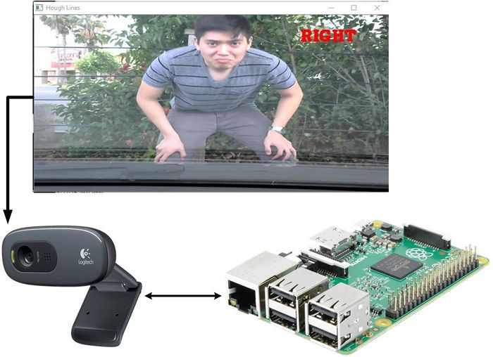
The Raspberry Pi 2 was chosen over the SJone Board because the SJone is incapable of doing image processing. The Raspberry Pi 2 runs an image of Linux called Raspbian Jessie. The Raspberry Pi 2 uses the BCM2836 (quad core ARMv7) chip running at 900 MHz.
A USB camera is used to provide video/image feed to the Raspberry Pi 2. The camera gives the Raspberry Pi 2 a peripheral of the real world surrounding and allow the Raspberry Pi 2 to do image processing of the input frames.
The Raspberry Pi 2 is powered on via USB port of the laptop. The USB camera is interfaced via USB as input to the Raspberry Pi 2 USB port.
 The USB camera can be turned on by using OpenCV API functions
 cv::VideoCapture cam = cv::VideoCapture("File path to video"); // Use a pre-recorded video
 cv::VideoCapture cam(1); // Turn on camera that is connected to USB port
Software Design
Below shows the basic algorithm on how lane detection can be achieved. The problem is that this will still produce a lot of noise, and intermediary steps must be done for proper lane detection.
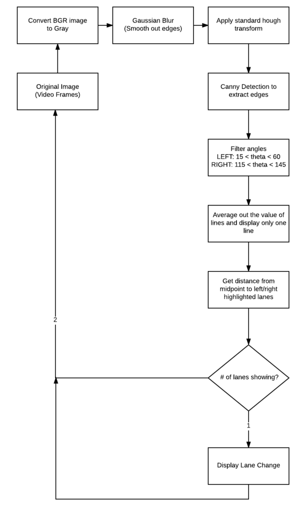
The flow chart below shows how the entire program was done. From filtering out noise to lane switching.
Implementation
OpenCV
OpenCV is an open source computer vision library that allows the programmer to utilize computer vision and machine learning software libraries for their projects. The library has more than 2500 optimized algorithms in its API. It supports many languages such as C++, C, Python, Java, etc.
In our project, we used OpenCV 3.1 and programmed in C++. The installation process of OpenCV on our laptops and Raspberry Pi 2s can take up to 5 hours. Documentation on how to setup OpenCV on different operating systems can be found on their official website. IDEs used to program are Eclipse and Visual Studios, in some cases makefiles were generated.
Color Spaces
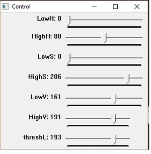
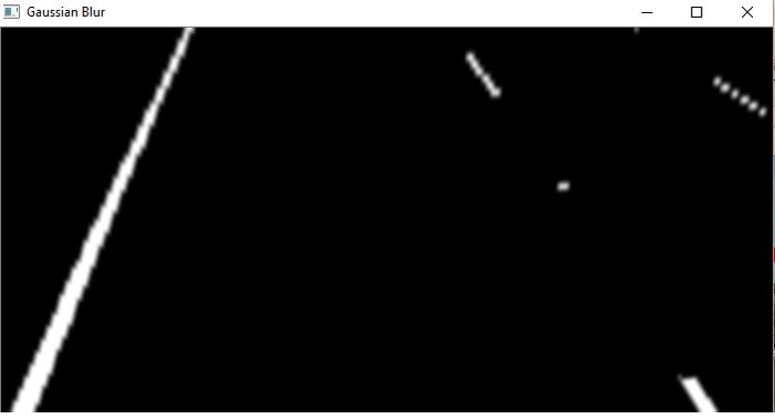
The images were converted from BGR (Blue Green Red) to grayscale. Canny edge detection needs to be done in gray scale. The grayscale image is then converted to HSV (Hue Saturation Value) so that we can use a trackbar to adjust the intensity of the image. We then binarize the image. Since images in grayscale are 8-bits per pixel, We then lower and higher value number between 0 to 255 to adjust the threshold. This will filter out noise.
IPM (Inverse Perspective Mapping)
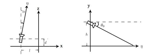
IPM can be thought of as a "bird's eye view" of the road. IPM transforms the perspective of 3-D space into 2-D space, therefore removing the perspective effect. Using this method is advantageous as it focuses directly on the lane marking instead of the surrounding environment. Therefore, reducing a lot of noise.
 Mat findHomography(InputArray srcPoints, InputArray dstPoints, int method=0, double ransacReprojThreshold=3, OutputArray mask=noArray() )
 // can be used to transform perspective from original to IPM
Although IPM was implemented and seemed promising, it was not used in the final version of the code. There was not enough time to further implement and transform/map the IPM coordinates back to the original video. Transforming IPM coordinates back to the original video can be done by:
 cv::getPerspectiveTransform(InputArray src, InputArray dst)   // to get the 3 x 3 matrix of a perspective transform
 cv::perspectiveTransform(inputVector, emptyOutputVector, yourTransformation)   // to transform the your IPM points to original video points
Although implemented and experimented, it was not able to map broken lane markings.
The above image shows the bird-eye view of the road after applying filters.
Contours
Using contour to detect lane markings was based on color and shape detection. When a rectangular shape is detected and color is detected, a rectangular box is drawn around the contour as detection. Color detection, in this case would be yellow and white, for lane markings, can be found by adjusting the HSV filter threshold values. The main disadvantage of using color detection is that there may be false positives present.
 Contours can be found using:
 void findContours(InputOutputArray image, OutputArrayOfArrays contours, OutputArray hierarchy, int mode, int method, Point offset=Point())
 cv::Mat drawing = cv::Mat::zeros(gaussian_image.size(), CV_8UC3);
 /* Draws a rectangle around the lanes */
 for (unsigned int i = 0; i < boundRect.size(); i++) {
    cv::rectangle(drawing, boundRect[i].tl(), boundRect[i].br(), cv::Scalar(0, 100, 255));
 }
Lane detection using contour was experimented and the result was promising, but the algorithm implemented was expensive and also used IPM, which was not able to be mapped back to its original points. The decision was then to focus on reducing noise from hough transform because it did not use IPM and seemed more efficient.
Gaussian Blur
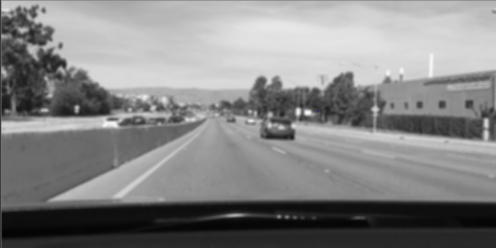
Gaussian Blur is used to blur out the image. is particularly useful to get rid of unwanted noise for the Canny edge. For example, clouds and trees all have numerous edges. By using Gaussian blur, we can make it seem like they don't have edges, so that Canny Edge detection won't detect the trees and clouds. Too much blur, and even the road's lines won't be traced out by the Canny Edge.
 cv::Size kSize = cv::Size(5, 5);
 cv::GaussianBlur(image, image, kSize, xSigma, ySigma);
Canny Edge
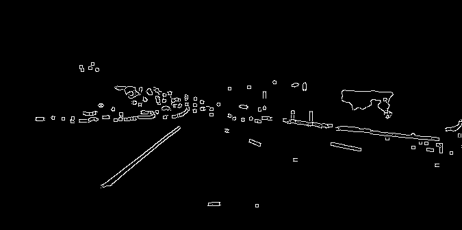
Canny edge is used to trace out edges of the image. The lane markings have an edge, and will be traced by this function. This new image is will then be used to generate Hough lines.
cv::Canny(gaussian_image, canny, upperThresh, lowerThresh);
Hough Line
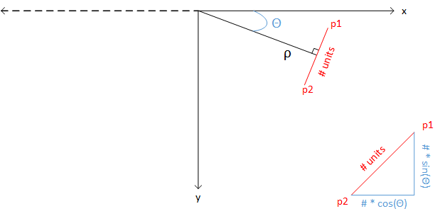
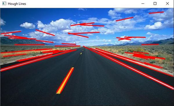
This is where the lane marking extraction occurs. A standard Hough line transform is used to highlight lane markings. In the videos, the slanted, vertical red lines are generated by the Hough function. Hough uses a voting system where it analyzes the data of the images and gathers a certain amount of "votes". The needed amount of votes needed to be considered a line is done using the threshold value of the HoughLine function. This may require some trial and error to determine. Too small of a value, there will be a large amount of noise, too big of a value, the lanes may not be detected. Theta is the angle of the line relative to the x-axis, and rho is the length of the line. Since lanes are slanted vertically from the perspective of the driver, theta (in degrees) is filtered to be 15 < theta < 60 for the left lane and 115 < theta < 145. Using this filter, horizontal lines will never be displayed since they aren't necessary. Multiple hough lines will be generated in the lane, so an average was calculated so only one line per lane will be shown.
Rho will go to the mid point of the line. The line will be perpendicular to rho. p1 and p2 are then adjusted to be a a certain amount of units away from the the middle (rho), and p1 and p2 are on opposite ends. p1 and p2 are then fed into the cv::line() function, and a line is drawn.
cv::HoughLines(canny_image, lines, rho, theta, threshold);
Percentage offset
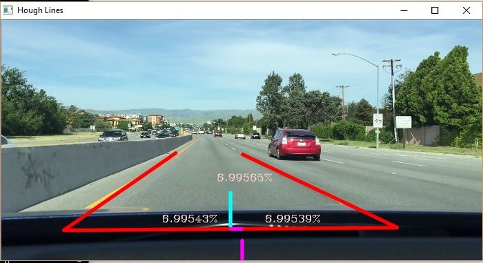
The percentage offset is used to determine how far away the center of the vehicle is from the center of the lane. The percentage offset is calculated when 2 lane markings are detected. It is calculated by using the distance formula (Pythagorean Theorem), using the closest points of the detected lane markings relative to the vehicle.
Three values are displayed:
The left value shows the percentage offset between the distances of left lane to center of lane boundary and to center of vehicle.
The center value shows the percentage offset between the distances from center of lane boundary and center of lane to to center of vehicle.
The right values shows the percentage offset between the distances of right lane to center of lane boundary and to center of vehicle.
Switching Lanes
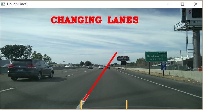
The typical time for an average driver to switch lane takes about one to three seconds. Using this time parameter, we can tell if the driver is switching lanes. The definition of switching lanes is when the driver departs from one lane boundary into another. When departing one lane boundary into another, only one lane will be detected by the camera. When only one lane is detected and within the time parameter, it will check if the lane marking is within a given boundary for it to be considered switching lanes.
Another method implemented to detect switching lanes is to measure the distance between the lane marking to the center of the vehicle (camera). As the distance decrease between a certain distance threshold and time, it will be considered switching lanes. The distance is also calculated using the distance formula.
Testing & Technical Challenges
Testing in a Dynamic Environment
The testing was done on a highway. Many adjustments to the HSV had to be done to get it right. There are many factors that could affect the test such as cars passing by and their shadows are over the lanes, making it hard to detect. Much of the test was done on sample videos before we took it out on the road. Every video had to have its HSV adjusted. Since OpenCV processes images frame-by-frame, testing on the road is no different than testing it on sample videos. It just takes a little more work to get the HSV values right because the colors could change at any moment.
General testing procedures include:
1) Adjusting HSV
2) Adjusting threshold and erosion
3) Adjusting thresholds of various functions such as canny() and HoughLine()
Issue 1: Noise
There are Large amounts of noise when generating Hough lines. This is because there are lines in each picture. Standard Hough lines do not work because you cannot set the minimum and maximum lengths of lines. Probabilistic Hough Lines are the best bet for this task. Even with Probabilistic Hough Lines, there is still quite a bit of noise.
Solution:
We did not use Probabalistic Hough Line. We used the standard one. Instead of using the Gaussian Blur, converting the image to HSV and then binarizing(threshold) it was sufficient. Adjusting HSV and threshold allows us to just the lanes. This is not perfect because there will still be some noise. To filter out more of the noise, we filtered out unnecessary horizontal angles because lanes from the driver point of view, is not horizontal, but slanted vertically. We filtered between the angles of 15 and 60 degrees for the left lane, and 115 and 145 degrees for the right lane. Erosion was also used to make the lanes appear thinner so we could get a better average.
Issue 2: Broken Lane Markings
Dotted lines are hard to deal with. Because Hough lines use a voting system, it's hard to find a proper a good point where it can detect dotted lanes without generating much noise.
A fix to this is to have an elapsed time where the lanes disappear. Because it takes time to change lanes, and the lines only disappear for a split second due to the speed of driving, we took made it so if the lines disappear for less than .3 seconds to continue on with the program. Only when the elapsed time is greater than .3 seconds do we deal with changing lanes.
Issue 3: Low Power CPU Image Processing Capability
Most of our development and testing was done on our own personal laptops, which can able to handle a lot of the image processing at a higher Frames/Second. We were worried about how much of a decrease in processing when porting our project over to the Raspberry Pi 2. When testing our code on the Raspberry Pi 2, there was a noticeable decrease in the Frames/Second.
Although there was a noticeable decrease in Frames/Second, it was still able to provide the same result as testing on our laptop and in a real and dynamic environment. We would recommend others to invest in a better SBC (Single Board Computer) with a GPU for image processing related projects.
Conclusion
Using OpenCV to detect lane markings and to notify lane changes was challenging. However it can potentially be a great way to detect lane markings as computers become cheaper. The bulk of the challenge comes from noise filtering and dotted lines. There are however, numerous amounts of variables to consider such as lighting, shadows, reflection from windows, weather conditions, roads with inconsistent lanes, etc. These are challenges that take a lot of time to fix. Computer vision can be used as an alternative to more expensive autonomous driving devices. We have learned a lot about raw image processing and computer vision. Computer vision is a vast field and we have only scraped the surface of it. Although the semester has ended, work on this project will continue.
Project Video
Project Source Code
References
Acknowledgement
Any acknowledgement that you may wish to provide can be included here.
References Used
HIPR2 Image Processing Learning Resources
Appendix
You can list the references you used.
